Problem

In 5022.htm you see a function combined of linear functions. How can you add steps to it which have changing widths and heights?

Solution (see also chart here)

Alternative 1: C1:
 =MIN(TRUNC(((A1-1%)%%-{0\0.2\0\0\0\0})/{0.1\0.3\1\2.5\5\25})*{8\6\15\16\11\7}+{10\42\72\4373\14868\24464},26137)
+SUMPRODUCT((ABS(A1%-{515\545\610\705\50050}-50%%%)<{15\15\10\5\50})*{9\3\6\3\1}) or

Alternative 2: B1: Insert Name Define "Charge" refers to:
=EVALUATE("=MIN(TRUNC((("&!A1&"-1%)%%"&CHOOSE(MATCH((!A1-1%)%%,{0\0.5\5\500\2500\5000})
,")/.1)*8+10","-.2)/.3)*6+42","))*15+72",")/2,5)*16+4373",")/5)*11+14868",")/25)*7+24464")&",26137)")+NOW()*0
B1: =Charge

(showing the fee of the notary public in Germany). See abbreviations here (German).

Remarks

The two alternative formulas have about the same length. Alternative 1 also runs on spreadsheets without named formulas.

The functions' steps are described by 4 parameters:
- shift on X-axis, here -{0\0.2\0\0\0\0} (needed, if steps of one of the combined formulas would not start at X=0)
- Y-axis point: here +{10\42\72\4373\14868\24464}
- height of steps: here *{8\6\15\16\11\7}
- width of steps: here  /{0.1\0.3\1\2.5\5\25}
At alternative 2, they are written as single formulas. Therefore, they appear in different order.

By using EVALUATE(), Alternative 2 (as a named formula) can be kept shorter than 4 VLOOKUP()s (one for each parameter, and each using {0\0.5\5\500\2500\5000} as lookup range) . It does not work in SpreadCE, which also requires Alternative 1 as array formula.

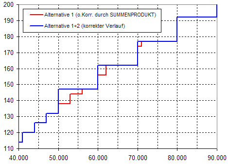
Alternative 1 follows 5022.htm, adding 2 parameters for the steps to those 2 for the linear functions. But still, it works wrong (expressed by the red line) without manual corrections by SUMPRODUCT() (blue line), see here:

What does it say? At over 50,000 Euro, each first cent of next 10,000 Euro cost us 15 Euro while before each first cent of next 3,000 Euro cost us 6 Euro. This means, that by continuing with steps' sizes below 50,000.01 Euro the red line would return the function's value, which would be wrong when it appeared -  this happening on some sections until 71,000 Euro. The blue line is prescribed by law. So, f(50,000.01) has to be corrected from 138 to 147 (+9, shown by {9\3\6\3\1}. f(5,000,000.01) until f(5,010,000) is outside of the chart, but has to be corrected by +1, the last array's entry. See the Excel file here.